Understanding HNSW: The Engine Behind Fast Vector Search

To understand HNSW, imagine walking into a library with millions of books, looking for a specific book based on a brief description of the content. If the books were all piled up randomly, you'd have to check every book individually to find the one that matches your description best, that's brute force. While it would eventually work, it would take forever.

But libraries aren't organized like that. They're structured to naturally guide you to the right section. You walk in and at the top level, you choose whether your book is in the fiction or nonfiction section. Then you narrow it down by genre history, science, or biography. After that, you move to more specific subcategories or alphabetical order until you reach the exact shelf where your book is located.

HNSW works the same way and that intuition is worth holding onto as we go deeper.

HNSW Indexing

HNSW (Hierarchical Navigable Small World) is a graph-based indexing algorithm used for Approximate Nearest Neighbor (ANN) search in high-dimensional vector spaces. Instead of comparing a query against every vector, HNSW organizes vectors into a hierarchical graph structure that enables fast navigation to the nearest neighbors.

The Building Blocks of HNSW

HNSW combines ideas from two powerful data structures: Navigable Small World (NSW) graphs and Skip Lists.

Building block 01

Navigable Small World (NSW)

A Navigable Small World is a type of network or graph that allows for efficient navigation and search through its nodes.

Structure

• Nodes represent data points (e.g., vectors)
• Edges represent connections between these points based on similarity

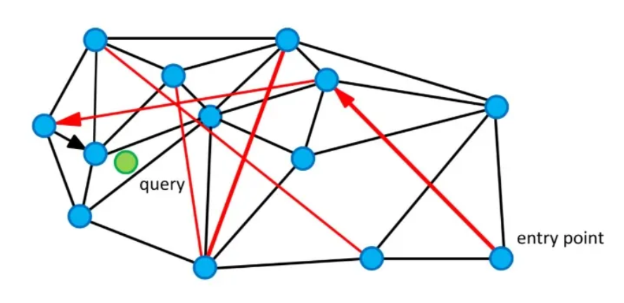
How NSW Search Works

• Each node is connected to other similar nodes
• The search starts from an entry point
• The algorithm repeatedly moves to neighboring nodes that appear closer to the query
• This allows efficient navigation instead of comparing the query against every vector

Limitation

Pure NSW can become trapped in local optima because it relies on greedy navigation. HNSW reduces this risk by using hierarchical layers and maintaining multiple candidate paths during search.

Local optimum: A node that appears to be the best choice within its immediate neighborhood, even though a better match exists elsewhere in the graph.

Building block 02

Skip Lists

A Skip List is a data structure that allows fast search, insertion, and deletion operations. It is essentially a multi-level linked list where each level allows "skipping" over multiple elements, reducing the time complexity of operations.

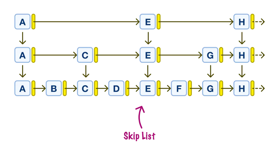
How Skip Lists Work

• Data is organized into multiple levels
• Higher levels contain fewer elements and act as shortcuts
• Instead of traversing everything step by step, the search can use these shortcuts to quickly reach the correct region
• Once near the target, the search switches to lower, more detailed levels

How HNSW Combines Both Ideas

HNSW merges these two concepts into a single structure:

• Uses the graph-based navigation of NSW to move between similar vectors
• Uses hierarchical layers inspired by Skip Lists to avoid getting trapped in poor search paths
• Higher layers provide a coarse overview of the dataset and help quickly locate the most promising region
• Lower layers contain denser connections that enable precise nearest-neighbor search

How Search Works in HNSW

The search process follows a top-down approach. Instead of starting with the full graph, the algorithm begins at the highest layer and gradually moves toward lower layers, refining its search at each step.

How Vectors Are Inserted into HNSW

Understanding how vectors are inserted is just as important as understanding how search works. The quality of the graph built during insertion directly determines how accurate and fast your searches will be later.

Step 1: Assigning a Maximum Layer

When a new vector arrives, HNSW first decides how high up in the hierarchy it will live. This is done by randomly drawing a maximum layer number using an exponential probability distribution. The result:

• Most vectors are assigned only to Layer 0
• Fewer vectors reach Layer 1
• Very few vectors reach Layer 2 or higher

This randomness is intentional because it's what naturally keeps upper layers sparse and lower layers dense, maintaining the hierarchical structure that makes HNSW fast.

Step 2: Finding the Entry Point (Top Layers)

Starting from the topmost layer of the graph, HNSW runs a greedy search, identical to the query search described earlier, moving toward nodes closest to the new vector. This phase has one goal: find the best entry point for the layer where insertion will actually happen. At each layer above the vector's assigned maximum, HNSW tracks only the single closest node and passes it down. No connections are formed yet.

Step 3: Selecting Neighbors (Insertion Layers)

Once HNSW reaches the vector's assigned maximum layer, the process changes. Instead of tracking just one candidate, it now tracks up to ef_construct candidates simultaneously. From these, HNSW selects the best m neighbors and creates bidirectional edges. This same process repeats going down through each layer until Layer 0.

This is the moment where the parameters you configure actually matter:

• ef_construct controls how many candidates are evaluated when choosing neighbors. A higher value means more options are considered, leading to better neighbor selections and a higher quality graph.
• m controls how many of those candidates actually become permanent connections. More connections means more paths available during future searches.

Why This Is Efficient

The key idea is that the upper layers act like shortcuts. Instead of searching the entire graph from the beginning, HNSW quickly identifies the correct region at higher levels and then performs increasingly detailed searches as it moves downward. Think of it like finding a book in a library:

• Layer 2 helps you find the correct floor
• Layer 1 helps you find the correct section
• Layer 0 helps you locate the exact shelf and book

By narrowing the search space at each layer, HNSW achieves extremely fast nearest-neighbor search while maintaining high accuracy.

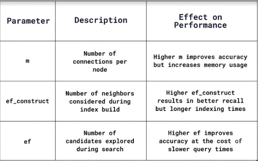
Configuring HNSW

You can fine-tune how the HNSW graph is built to balance search speed, accuracy, memory usage, and indexing time depending on your use case. There are three key parameters: m, hnsw_ef, and ef_construct.

Why HNSW Is Fast and Scalable

Sublinear Search Scaling

Unlike O(N) brute force search, HNSW search grows roughly logarithmically with the number of vectors. This makes million-scale datasets searchable in milliseconds rather than minutes.

Filter-Aware

Qdrant extends HNSW with filter-aware indexing (Filterable HNSW), allowing fast searches under structured conditions. This avoids costly full scans when filtering by metadata.

Large-Scale Use

• Supports real-time updates while maintaining high recall
• Fits semantic search and recommendation systems
• Scales from thousands to billions of vectors

HNSW is one of the key innovations that made modern vector search practical at scale. Instead of comparing a query against millions of vectors, it intelligently navigates a hierarchical graph to quickly reach the most relevant results. By combining the navigability of small-world graphs with the hierarchical shortcuts of skip lists, HNSW delivers an impressive balance of speed, accuracy, and scalability.

Whether you're building semantic search, recommendation systems, RAG applications, or large-scale AI products, chances are an HNSW graph is working behind the scenes to make those millisecond searches possible. The next time a vector database returns relevant results almost instantly, you'll know it's not magic — it's smart graph navigation.