The Universal Query API: How Multi-Stage Retrieval Solves the Speed vs. Accuracy Tradeoff
1. Introduction
Anyone who has built a search or retrieval system eventually runs into the same wall: fast methods aren't accurate enough, and accurate methods aren't fast enough. Single vector embeddings can scan millions of documents in milliseconds, but they miss nuance. Multi-vector methods like MaxSim capture that nuance, but running them over an entire collection is computationally expensive.
The instinct to pick one approach and live with its tradeoffs is understandable, but it isn't necessary. Modern retrieval systems increasingly rely on multi-stage pipelines that combine both: a fast approximate stage to narrow the field, followed by a precise stage to rerank what's left.
This is the idea behind Qdrant's universal query API. It packages the entire prefetch-and-rerank pattern into a single call, so you get the speed of approximate search and the precision of exhaustive scoring without having to build and glue together the two stages yourself. This article walks through how that pattern works, why oversampling is the detail that makes it actually reliable, and how to implement it.
2. The Core Tension
The most effective production deployments don't rely on a single retrieval method. They combine multiple techniques in multi-stage pipelines.
Fast approximate methods retrieve candidates. Then higher quality methods rerank only those candidates. This pattern solves a fundamental tension in search system design: single vector search is fast but less accurate, while multi vector search is accurate but computationally intensive.
Multistage retrieval gives you both the speed of approximate search and the precision of max similarity search.
3. How the Universal Query API Works
Qdrant's universal query API makes building sophisticated retrieval pipelines straightforward. The core pattern is simple. At the first stage, fast single vector retrieval using HNSW pulls, say, 500 candidates in milliseconds. This narrows the search space dramatically from potentially millions of documents.
Then precise maximum similarity (MaxSim) ranking is applied on those candidates. It uses the full quality of multi vector scoring to arrive at, say, the top 10 results.
Stage 1: Fast single-vector retrieval (HNSW) → 500 candidates
Stage 2: Precise MaxSim reranking → top 10 results
1M documents × MaxSim → 500 × MaxSim = a 2000x reduction in the number of comparisons the expensive scoring step needs to perform.
The result is similar final quality but at a fraction of the cost. You get instant initial retrieval plus high quality reranking, all in a single query.
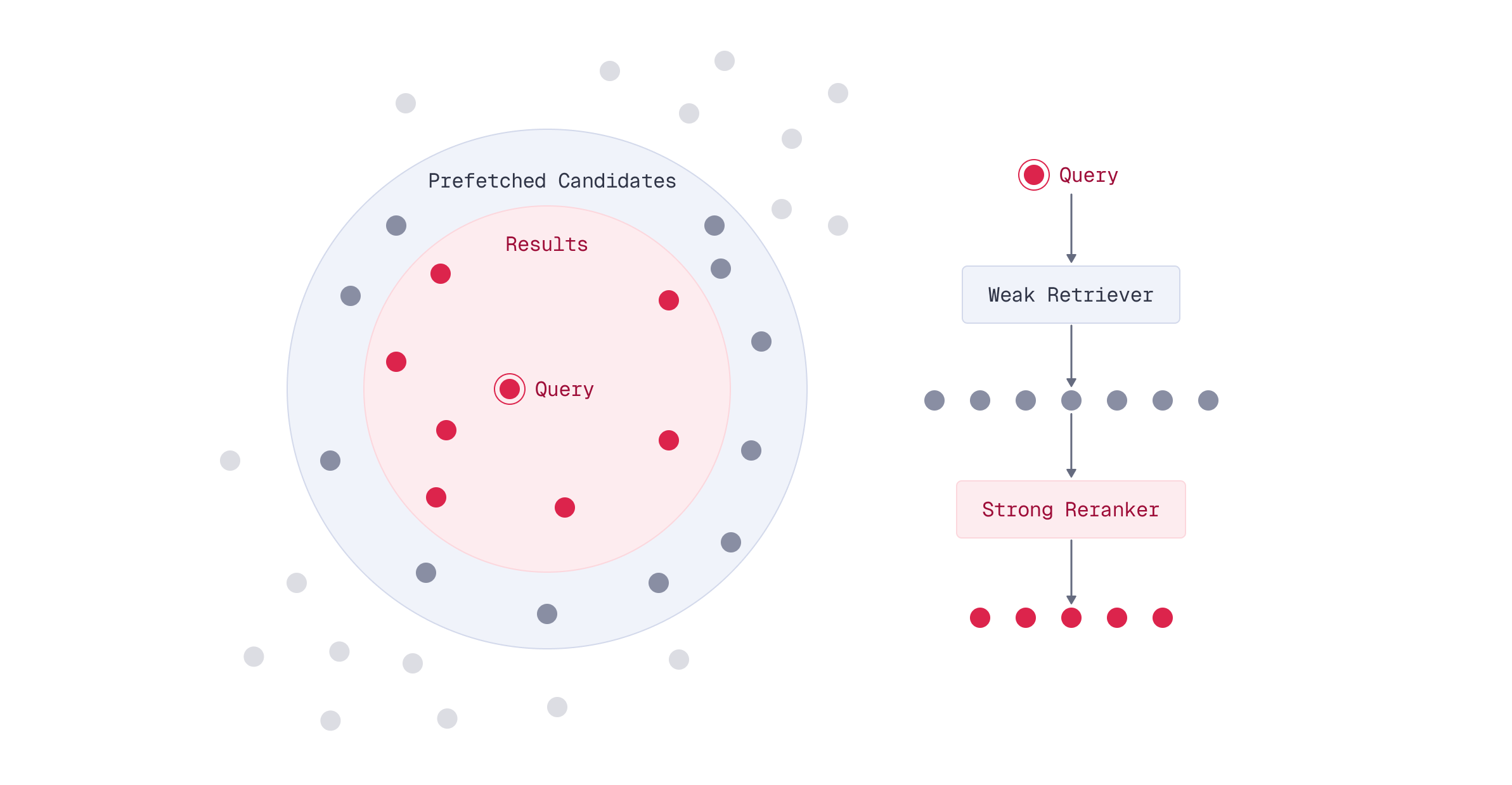
This diagram shows how this works. Millions of documents narrow to hundreds of candidates narrow to your final results. Each stage uses the right tool for your job. HNSW for speed, MaxSim for precision.
4. Why Oversampling Is Non-Negotiable
There is one key aspect that makes this whole pattern work: you must retrieve more candidates in the prefetch stage than you want in your final results. This is called oversampling, and it's non-negotiable for maintaining quality.
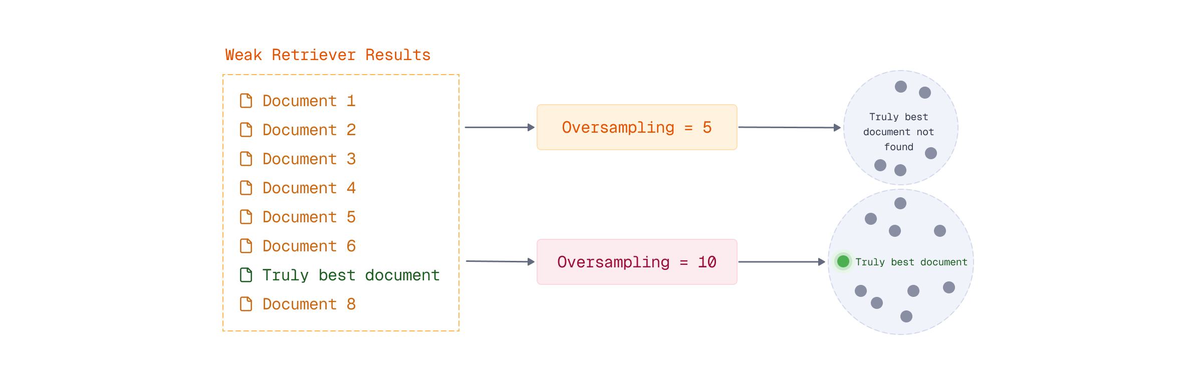
Without oversampling, you are capped at single vector quality. If the truly best document according to MaxSim was ranked 11th by the fast method, and you only asked for 10 documents to be returned, MaxSim never sees it. You've limited yourself to whatever the single vector model happened to select.
With oversampling, the truly best documents have a chance to surface. You cast a wider net, then pick the best fish. Documents that weren't even at the very top of the single vector ranking can still make it into your final results.
4.1 Oversampling in Practice
Consider a ranked list of candidates where the truly best document sits somewhere in the middle of the pack. With an oversampling factor of 5, the retrieval window may be too narrow to include it, and the truly best doc is never found. With an oversampling factor of 10, the window widens enough to capture it.
This illustrates how recall improves with higher oversampling. More candidates mean more chances to capture the right documents before reranking.
The curve typically shows diminishing returns. Going from 100 to 500 candidates helps more than going from 500 to 1000, since the early gains in oversampling are the cheapest ones to buy.
4.2 Choosing an Oversampling Factor
The oversampling factor, how many candidates you retrieve versus how many final results you want, is itself a trade-off, not a free lunch.
Higher oversampling (e.g., retrieve 1000 to return 10) gives you better final search quality, at the cost of more computation in the reranking stage.
Lower oversampling (e.g., retrieve 50 to return 10) gives you a faster, cheaper query, but with a real risk of missing relevant documents that the fast stage ranked just outside the window.
There's no universally correct number here. It depends on how much you trust your fast retriever and how much latency and compute budget you're willing to spend on the rerank.
5. Implementing the Pipeline in Qdrant
Qdrant makes it easy to implement this kind of pipeline through four building blocks.
5.1 Dual Representations
Store both single-vector and multi-vector representations for the same document. Each document gets both a fast single index vector and a multi-vector representation for precise scoring.
5.2 The Prefetch Array
You use the prefetch array for stage 1. It lets you specify the single vector named vector, the limit of how many candidates to retrieve, and the model to use for encoding the query.
5.3 The Main Query
The main query handles stage 2: multi-vector MaxSim scoring against only the prefetch candidates. This is where precision matters.
5.4 One API Call, One Pipeline
One API call does everything. Qdrant executes the entire pipeline server side. Prefetch runs first with fast HNSW. Then the main query ranks only those candidates using max similarity.
Multi-stage retrieval dramatically reduces computational cost while maintaining quality. Instead of running MaxSim against millions of documents, you compute MaxSim against hundreds. The speedup is roughly collection size divided by candidate count: a collection of 1M documents with a prefetch of 1000 candidates means roughly 1000x fewer MaxSim calculations than scoring every document directly. A smaller collection of 100K documents with a prefetch of 500 candidates still gets you roughly 200x fewer calculations. Higher oversampling improves quality but increases how much work Stage 2 has to do, so the right number is a balance, not a fixed rule.
What This Looks Like in Code
The four building blocks above map almost directly onto a single query_points call. Here's a minimal example: a fast single-vector model handles the prefetch, and ColBERT reranks with MaxSim.
results = client.query_points(
    collection_name="hybrid-search",
    prefetch=[
        models.Prefetch(
            query=models.Document(
                text=query,
                model="BAAI/bge-small-en-v1.5",
            ),
            using="bge-small-en-v1.5",
            limit=500,  # oversampling: candidates for reranking
        ),
    ],
    query=models.Document(
        text=query,
        model="colbert-ir/colbertv2.0",
    ),
    using="colbert",
    limit=10,  # final results after reranking
)
Everything else, embedding the query, running HNSW search, scoring with MaxSim, happens server-side in one round trip.
Worth keeping in mind: multi-vector representations are memory intensive, storing a thousand vectors per document adds up quickly at scale, which is part of why this pattern matters. Keeping a fast single-vector index alongside the multi-vector one isn't just a speed optimization; it's what makes multi-vector search viable at all once your collection gets large.
6. Advanced Multi-Stage Patterns
The two-stage pattern covers most cases, but the prefetch mechanism is more flexible than that.
6.1 Chaining More Than Two Stages
Multi-stage retrieval isn't limited to exactly two stages. Because a prefetch can itself contain nested prefetch operations, you can chain three or more stages, each one narrowing the candidate pool further before handing it off to the next, progressively more expensive, method.
6.2 Combining Multiple Weak Retrievers
You can also run more than one retrieval method inside the prefetch stage itself. A common pattern is combining dense vectors with sparse BM25 vectors through query fusion, producing a stronger initial candidate set than either method would on its own, and then reranking the fused result with ColBERT.
This hybrid prefetch approach tends to improve recall: it helps ensure the candidate pool contains relevant documents that might otherwise be missed by dense or sparse search alone.
# Multi-stage with hybrid prefetch: combine dense and sparse retrieval
results = client.query_points(
    collection_name="hybrid-search",
    prefetch=[
        # Dense retrieval using single-vector embeddings
        models.Prefetch(
            query=models.Document(
                text=query,
                model="BAAI/bge-small-en-v1.5",
            ),
            using="bge-small-en-v1.5",
            limit=500,
        ),
        # Sparse retrieval using BM25
        models.Prefetch(
            query=models.Document(
                text=query,
                model="Qdrant/bm25",
            ),
            using="bm25",
            limit=500,
        ),
    ],
    # Results from both prefetch queries are combined, then reranked
    query=models.Document(
        text=query,
        model="colbert-ir/colbertv2.0",
    ),
    using="colbert",
    limit=10,
)
6.3 Filters Propagate Automatically
One detail worth knowing before you build this in production: filters applied to the main query automatically propagate to every prefetch stage. If you filter the main query by category or date, that same filter narrows the candidate pool from the very first stage, not just the final rerank.
This is efficient by design. Narrowing the pool early reduces computational cost throughout the entire pipeline, rather than filtering only after the expensive reranking step has already run.
7. When to Use Multi-Stage Retrieval
Multi-stage retrieval isn't free to build and maintain, so it's worth knowing when it actually pays off.
It's valuable for large collections, roughly 100K documents and up, where you need fast queries while still preserving multi-vector quality. It's especially effective when you're combining different embedding models or actively trying to reduce compute costs at scale.
It's worth skipping for small collections (under 10K documents), cases where single-vector embeddings are already good enough, or real-time indexing scenarios where maintaining dual embeddings adds more overhead than the pipeline saves you.
8. Conclusion
Single vector search and multi vector search aren't competitors. They're complementary tools that solve different halves of the same problem, and multi-stage retrieval, done through prefetch-and-rerank with sensible oversampling, is how you get the speed of one and the precision of the other without paying the full cost of either.
It's also just one tool among several, alongside score boosting, diversification, filtering, and query fusion, all composable into a single Qdrant request. There's no one configuration that's right for every system: the best pipeline depends on your data, your quality bar, and your budget, which is why evaluating different configurations matters as much as the architecture itself.